Approximating Pi using the Tau Manifesto
Because it's funny.
I started writing this post ten days ago when I realised Pi Day was approaching. Much like how people panic-buy in anticipation of a shortage, this post is very much the product of some last-minute panic writing.
With that said, let’s approximate \(\pi\) using the Tau Manifesto. Why, you ask? Because it’s the silliest way to celebrate Pi Day that I can possibly think of.
The three puzzle pieces
Accomplishing this requires three apparently unconnected concepts: the Basel problem, the Tau Manifesto, and the Zipf-Mandelbrot law.
The first piece of the puzzle: The Basel Problem
The Basel problem concerns the following infinite summation.
\[\sum^{\infty}_{n=1} \frac{1}{n^2} = 1 + \frac{1}{2^2} + \frac{1}{3^2} + \frac{1}{4^2} \cdots =\; ?\]In 1734, Leonard Euler showed that this infinite sum converges to exactly \(\pi^2 / 6\), which makes it a great candidate for \(\pi\) approximation. We can rewrite this formula by replacing reciprocals of squares with squares of reciprocals:
\[\begin{alignat*}{3} \sum^{\infty}_{n=1} \frac{1}{n^2} &= 1 + \frac{1}{2^2} + \frac{1}{3^2} + \frac{1}{4^2} + \cdots &= \frac{\pi^2}{6}\\ &\Downarrow\\ \sum^{\infty}_{n=1} \left(\frac{1}{n}\right)^2 &= 1 + \left(\frac{1}{2}\right)^2 + \left(\frac{1}{3}\right)^2 + \left(\frac{1}{4}\right)^2 + \cdots &= \frac{\pi^2}{6} \label{eq:basel}\tag{1} \end{alignat*}\]The second piece of the puzzle: The Tau Manifesto
In June 2010, American physicist Michael Hartl published the famous Tau Manifesto, in which he claims the following:
The natural choice for the circle constant is the ratio of a circle’s circumference not to its diameter, but to its radius.
(from The Tau Manifesto)
In other words, Hartl argues that it is more reasonable to use the constant
\[\tau = \frac{\text{circumference}}{\text{radius}} = 6.28318\cdots\]than the more familiar
\[\pi = \frac{\text{circumference}}{\text{diameter}} = 3.14159\cdots\]when working with geometry, analysis, physics, and just mathematics in general.
I won’t delve too deep into the unbelievably controversial (and surprisingly still relevant) \(\pi\) versus \(\tau\) debate, although the manifesto itself is quite an entertaining and fascinating read. Its PDF version spans a total of 53 pages, and its contents have been revised multiple times since its original publication. In this post, I will be using the latest version of the document, last updated on Tau Day 2023.
The third piece of the puzzle: The Zipf-Mandelbrot law for letter frequencies
So far our two puzzle pieces appear completely unrelated: one illustrates a problem from maths, one suggests a problem with maths. To link them, we will introduce the third and last piece of the puzzle: the Zipf-Mandelbrot law.
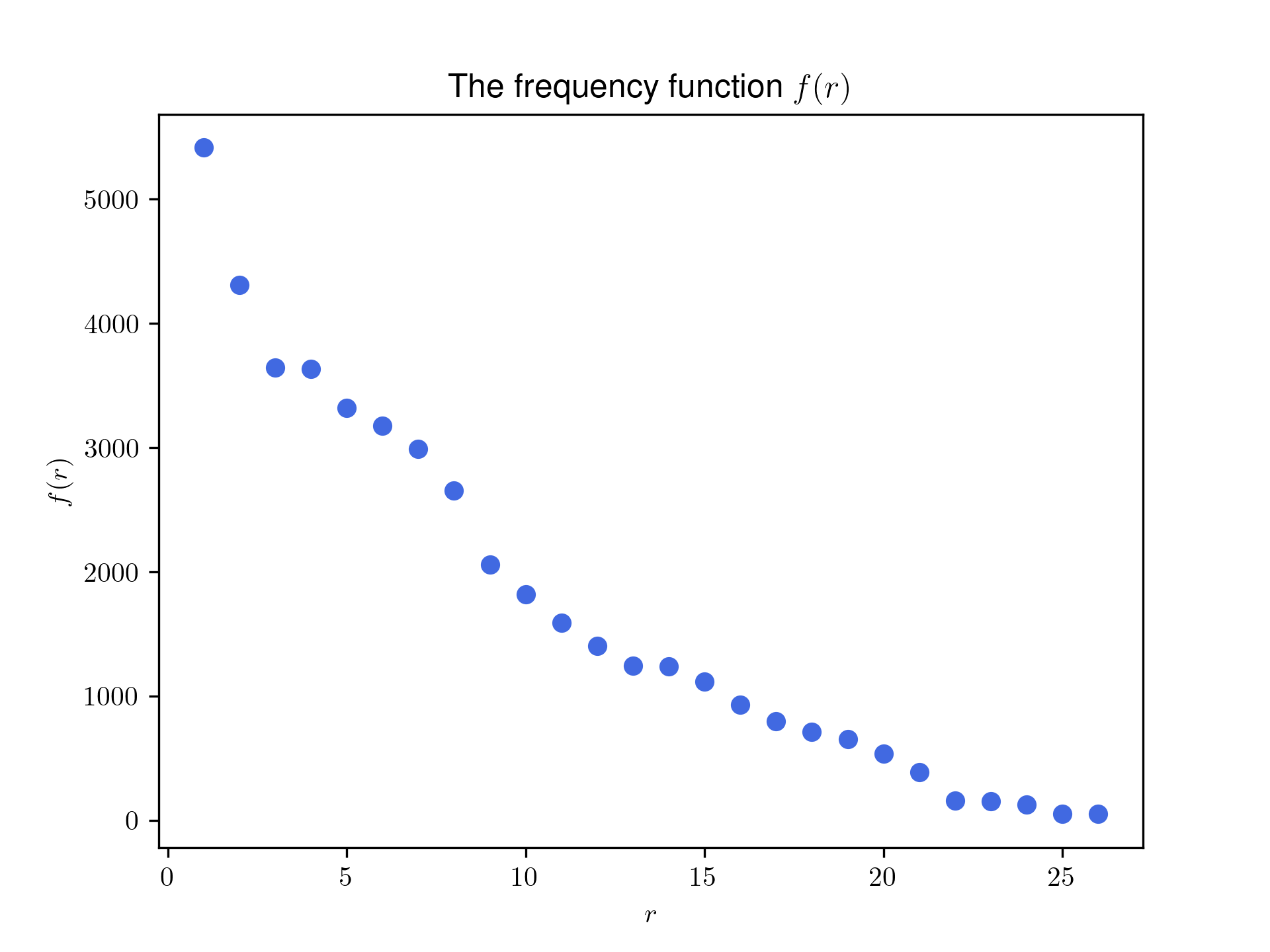
Given a large piece of written text, let us count the number of times each letter is used throughout. We denote the number of times the \(r\)-th most common letter appears by \(f(r)\), which we will call the frequency function. (Here \(r\) stands for “rank” or “ranking”.)
In quantitative linguistics, Zipf’s law refers to the empirical observation that \(f(r)\) decreases with \(r\) in a roughly hyperbolic manner, i.e.
\[f(r) \propto \frac{1}{r}\]where \(r = 1, 2, 3, \cdots\).
This means that the most commonly used letter should appear approximately…
- twice as often as the second most common letter,
- three times as often as the third most common letter,
- four times as often as the fourth most common letter,
- and so on.
It should be noted that in reality, Zipf’s law applies to not just letter frequencies, but word frequencies as well. This Wolfram demonstration, for example, uses logarithmic plots to illustrate how the word and letter frequencies of various literary works follow — or deviate from — Zipf’s law.
Being merely empirical, Zipf’s law is never entirely accurate. Real-world data may not always match its predictions, making it challenging to model language usage based on the law. To improve modelling accuracy, a 1953 paper by Benoit Mandelbrot proposes what is now called the Zipf-Mandelbrot law:
\[f(r) \propto \frac{1}{(r+\beta)^\alpha} \label{eq:zipf-mandelbrot}\tag{2}\]where \(\alpha\) and \(\beta\) are constants that can be adjusted based on the specific language and text in question. For instance:
- Setting \(\alpha = 1\) and \(\beta = 0\) gives the original Zipf’s law.
- It is suggested that setting \(\alpha = 1\) and \(\beta = 2.73\) yields the best fit for modelling word frequencies in American English.
I can’t find any sources mentioning the ideal parameter values for modelling the frequencies of English letters, but for the purposes of this post we will assume that the second set of parameters mentioned above, i.e. \((\alpha, \beta) = (1,\; 2.73)\), will work just as well for letter frequencies.
Manipulating the Zipf-Mandelbrot law
Now that we’ve acquainted ourselves with all three tools, let us begin by manipulating the Zipf-Mandelbrot law. (A lot.)
If we substitute \(\alpha = 1\) into \(\eqref{eq:zipf-mandelbrot}\), we get
\[f(r) \propto \frac{1}{r+\beta}\]which we can rewrite as
\[f(r) = \frac{k}{r+\beta} \tag{3}\label{eq:freq-func-def}\]for some nonzero constant \(k\). We’ll leave \(\beta = 2.73\) unsubstituted for now.
Setting \(r = 1\) gives us
\[\begin{align*} f(1) &= \frac{k}{1 + \beta}\\ k &= (1 + \beta) \cdot f(1) \end{align*}\]so
\[\begin{align*} f(r) &= \frac{(1 + \beta) \cdot f(1)}{r + \beta}\\ \frac{f(r)}{(1 + \beta) \cdot f(1)} &= \frac{1}{r + \beta}\\ \frac{f(r - \beta)}{(1 + \beta) \cdot f(1)} &= \frac{1}{r} \tag{replacing $r$ with $(r-\beta)$}\\ \frac{1}{r} &= \frac{f(r - \beta)}{(1 + \beta) \cdot f(1)} \end{align*}\]This means that for any \(r\), we can estimate its reciprocal \(1/r\) by evaluating the function
\[R_{\text{est}}(r) := \frac{f(r - \beta)}{(1 + \beta) \cdot f(1)} \tag{4}\label{eq:reciprocal-approx}\](\(R_{\text{est}}\) stands for “estimate of reciprocal”.)
There’s just one slight issue. Recall that \(r\), which stands for the rank of a certain letter, is an integer. On the left-hand side, \(r\) is used as the argument of the function \(R_{\text{est}}\), which is fine since the domain of \(R_{\text{est}}\) is the set of real numbers. The right-hand side, however, applies the frequency function \(f\) to a non-integer value \(r - \beta = r - 2.73\). Since \(f\) is defined only on positive integers, this is an invalid operation.
We can fix this by extending the domain of \(f\). Suppose we know the values of \(f(r_0)\) and \(f(r_0 + 1)\) for some integer \(r_0\). How can we infer from this the value of \(f(r_0 + t)\) for any \(0 \leq t \leq 1\)?
For starters, we know from \(\eqref{eq:freq-func-def}\) that
\[\begin{align*} f(r_0) &= \frac{k}{r_0 + \beta}\\ f(r_0 + 1) &= \frac{k}{r_0 + 1 + \beta} \end{align*}\]It follows that
\[\begin{align*} r_0 &= \frac{k}{f(r_0)} - \beta\\ r_0 + 1 &= \frac{k}{f(r_0 + 1)} - \beta \end{align*}\]With a bit of rearranging, we can combine these two equations to get the following.
\[\begin{align*} r_0 + t &= \frac{k}{f(r_0)} - \beta + t \left(\left(\frac{k}{f(r_0 + 1)} - \beta\right) - \left(\frac{k}{f(r_0)} - \beta\right)\right)\\ &= \frac{k}{f(r_0)} - \beta + t \left(\frac{k}{f(r_0 + 1)} - \frac{k}{f(r_0)}\right) \end{align*}\]Applying \(f\) to both sides, we have
\[\begin{align*} f(r_0 + t) &= \frac{k}{\frac{k}{f(r_0)} - \beta + t \left(\frac{k}{f(r_0 + 1)} - \frac{k}{f(r_0)}\right) + \beta}\\ &= \frac{k}{\frac{k}{f(r_0)} + t \left(\frac{k}{f(r_0 + 1)} - \frac{k}{f(r_0)}\right)}\\ &= \frac{1}{\frac{1}{f(r_0)} + t \left(\frac{1}{f(r_0 + 1)} - \frac{1}{f(r_0)}\right)}\\ \end{align*}\]We can simplify this equation using the linear interpolation (LERP) formula.
\[f(r_0 + t) = \frac{1}{\text{lerp}\left(\frac{1}{f(r_0)},\; \frac{1}{f(r_0 + 1)},\; t\right)}\]This allows us to extend the domain of \(f\) to \(\{r \in \mathbb{R} \;\vert\; r \geq 1\}\), as shown below.
\[f(r) = \begin{cases} \text{number of times the $r$-th most common letter appears} & \text{if $r \in \mathbb{N}$}\\ &\\ \dfrac{1}{\text{lerp}\left(\frac{1}{f(\lfloor r \rfloor)},\; \frac{1}{f(\lceil r \rceil)},\; r - \lfloor r \rfloor\right)} &\text{otherwise} \end{cases} \tag{5}\label{eq:freq-func-def-extended}\]This also restricts the domain of \(R_{\text{est}}(r)\), as defined in \(\eqref{eq:reciprocal-approx}\), to \(\{r \in \mathbb{R} \;\vert\; r \geq 1 + \beta\}\).
With all that done, it’s time to finally derive the formula we will use for our \(\pi\) approximation.
Crafting the formula
Combining all of the above, we have
\[\begin{align*} \frac{\pi^2}{6} &= \sum^{\infty}_{r=1} \left(\frac{1}{r}\right)^2 \tag{from \eqref{eq:basel}}\\ &\approx \sum^{26}_{r=1} \left(\frac{1}{r}\right)^2 \tag{partial sum}\\ &= \sum^{3}_{r=1} \left(\frac{1}{r}\right)^2 + \sum^{26}_{r=4} \left(\frac{1}{r}\right)^2\\ &= \sum^{3}_{r=1} \left(\frac{1}{r}\right)^2 + \sum^{26}_{r=4} (R_{\text{est}}(r))^2\\ &= 1 + \frac{1}{4} + \frac{1}{9} + \sum^{26}_{r=4} \left(\frac{f(r - \beta)}{(1 + \beta) \cdot f(1)}\right)^2 \tag{from \eqref{eq:reciprocal-approx}} \end{align*}\]where \(\beta = 2.73\) and \(f\) is defined in accordance with \(\eqref{eq:freq-func-def-extended}\). Note that the first three terms of the partial sum have to be calculated separately because \(R_{\text{est}}(r)\) is defined only in the domain of \(\{r \in \mathbb{R} \;\vert\; r \geq 1 + \beta = 3.73\}\).
The estimation
Now to actually evaluate this formula with regard to The Tau Manifesto! To do this, we can extract the contents of the document by scraping and parsing its official website’s HTML source code. This gives us a bunch of raw text that looks a bit like this. (Below shows the raw text corresponding to the opening lines of the manifesto’s first subsection.)
1.1 An immodest proposal
We begin repairing the damage wrought by \( \pi \) by first understanding the notorious number itself. The traditional definition for the circle constant sets \( \pi \) equal to the ratio of a circle’s circumference (length) to its diameter (width):2
\begin{equation}
\label{eq:pi}
\pi \equiv \frac{C}{D} = 3.14159265\ldots
\end{equation}
The number \( \pi \) has many remarkable properties—among other things, it is irrational and indeed transcendental—and its presence in mathematical formulas is widespread.
As we can see, the document uses a lot of LaTeX code to render mathematical expressions and equations. To prevent these from skewing the results, I used a few regular expressions to detect and remove all traces of LaTeX, leaving us with the following.
1.1 An immodest proposal
We begin repairing the damage wrought by  by first understanding the notorious number itself. The traditional definition for the circle constant sets  equal to the ratio of a circle’s circumference (length) to its diameter (width):2

The number  has many remarkable properties—among other things, it is irrational and indeed transcendental—and its presence in mathematical formulas is widespread.
Lastly, I removed all numbers, punctuation and newline characters, before converting everything to lowercase:
an immodest proposal we begin repairing the damage wrought by by first understanding the notorious number itself the traditional definition for the circle constant sets equal to the ratio of a circles circumference length to its diameter width the number has many remarkable properties among other things it is irrational and indeed transcendental and its presence in mathematical formulas is widespread
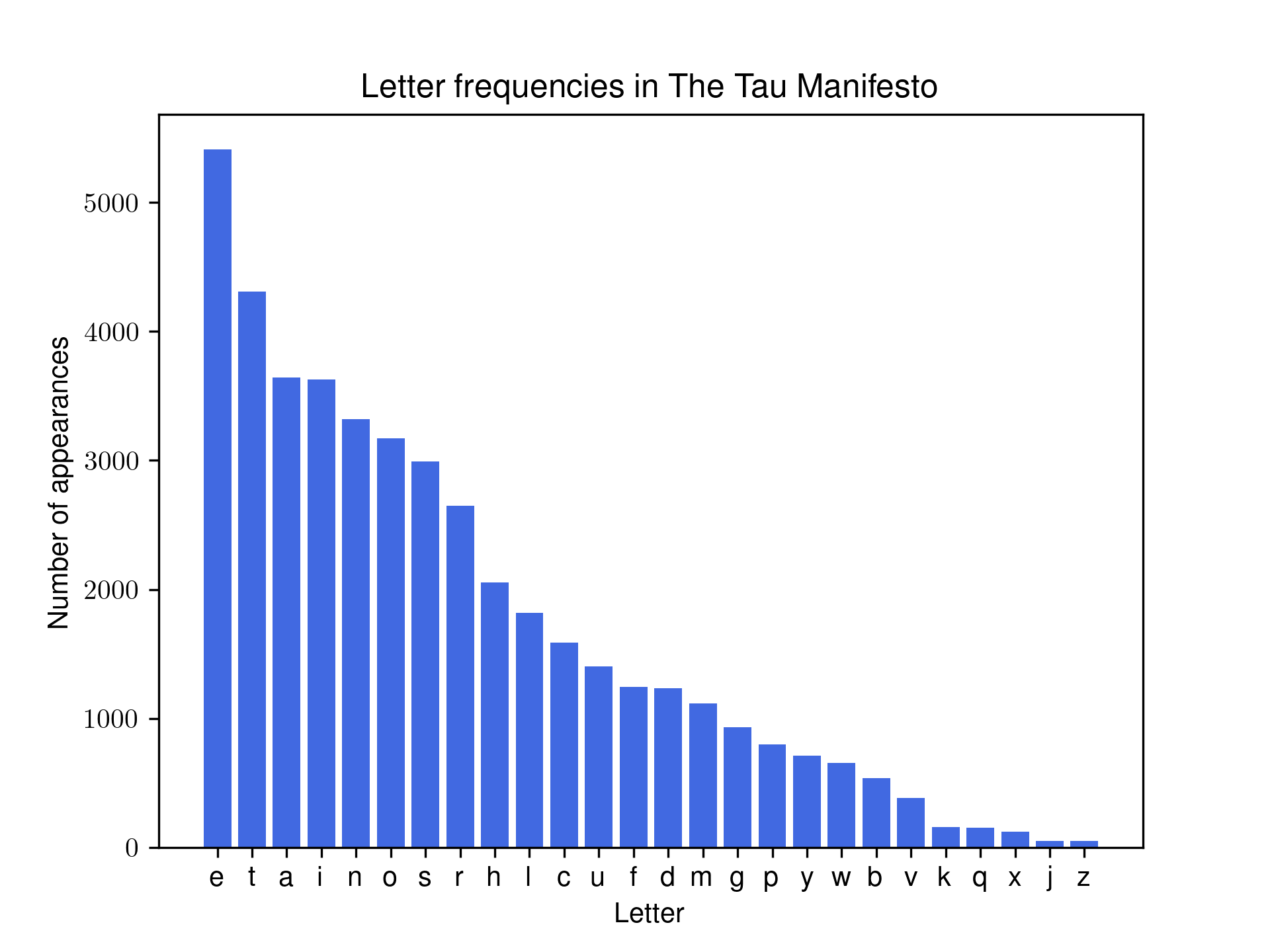
We can then run a simple letter frequency counter on the pre-processed text:
This enables us to plot a graph of \(R_{\text{est}}(r)\), displayed below.
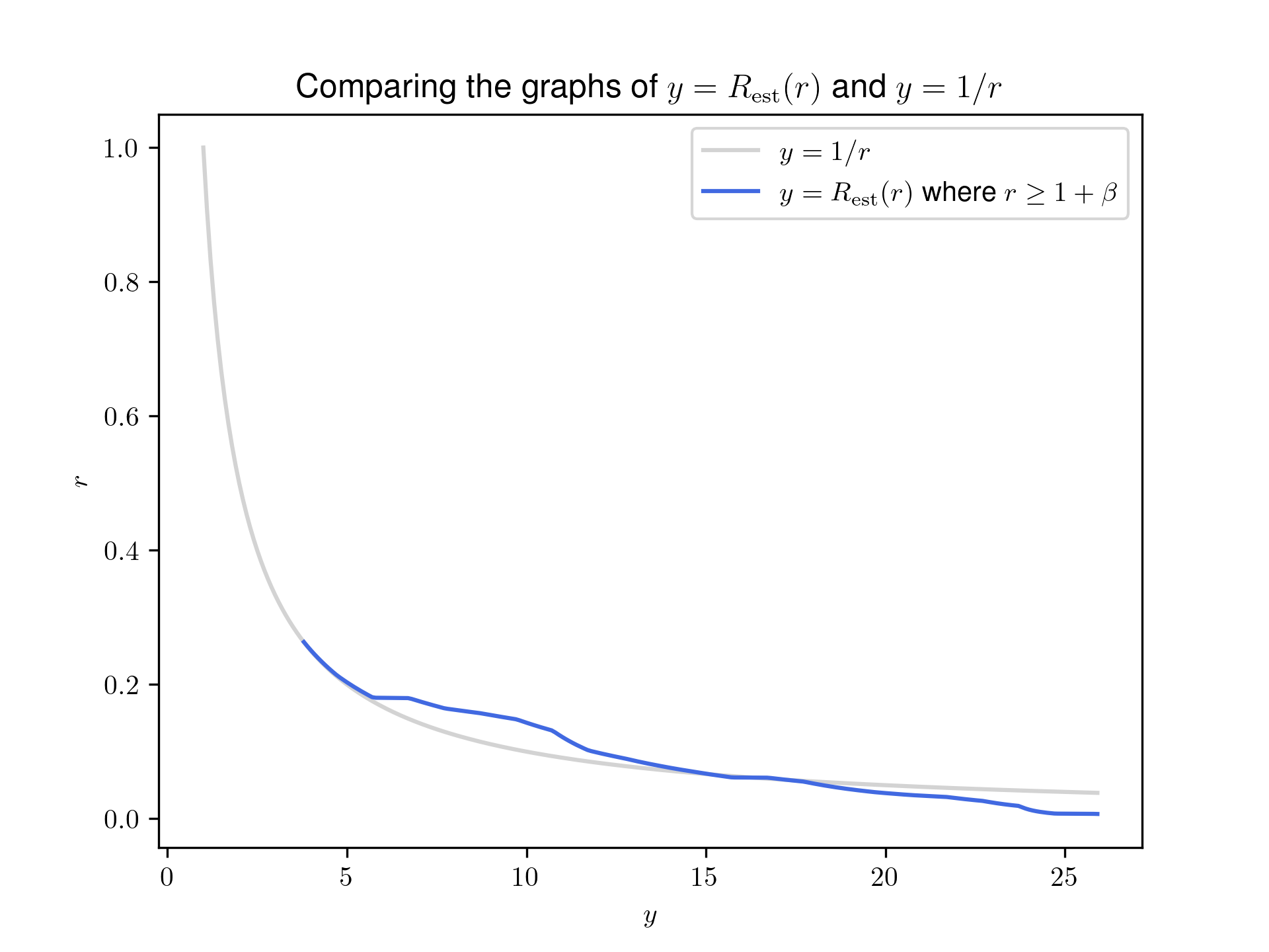
That’s a pretty decent approximation!
And now, all that’s left to do is to plug in every single value of \(r\) from \(4\) to \(26\):
\[\begin{align*} \frac{\pi^2}{6} &\approx 1 + \frac{1}{4} + \frac{1}{9} + \sum^{26}_{r=4} (R_{\text{est}}(r))^2\\ &= 1 + \frac{1}{4} + \frac{1}{9} + \sum^{26}_{r=4} \left(\frac{f(r - \beta)}{(1 + \beta) \cdot f(1)}\right)^2\\ &= 1.6579610987027469 \cdots \end{align*}\]and — for the finale — rearrange the equation to get:
\[\pi = 3.154008020315814 \cdots\]Honestly, with a percentage error of merely \(0.395\%\), that is a whole lot closer than I expected. Happy \(\pi\) day everyone!